emsa-analyzer.com · quick guide

EMSA Analyzer

how to get a K_d from a gel image, step by step

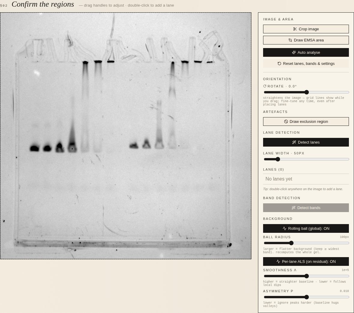
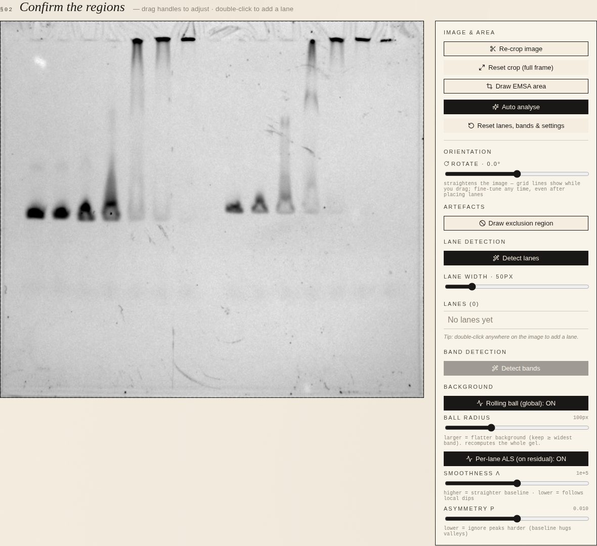
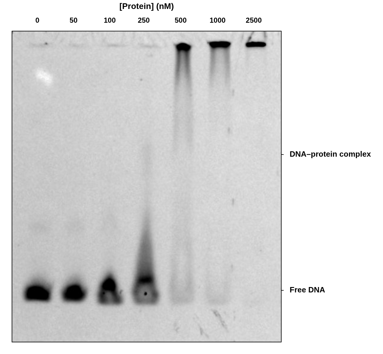
Every screenshot below comes from one example gel: two titrations side by side, each 0 · 50 · 100 · 250 · 500 · 1000 · 2500 nM left to right. The bound complex sits in the wells and smears below them; the free probe runs near the bottom. Nothing is placed for you — you confirm every region.

Prepare the image

EMSA analysis tab

01Upload

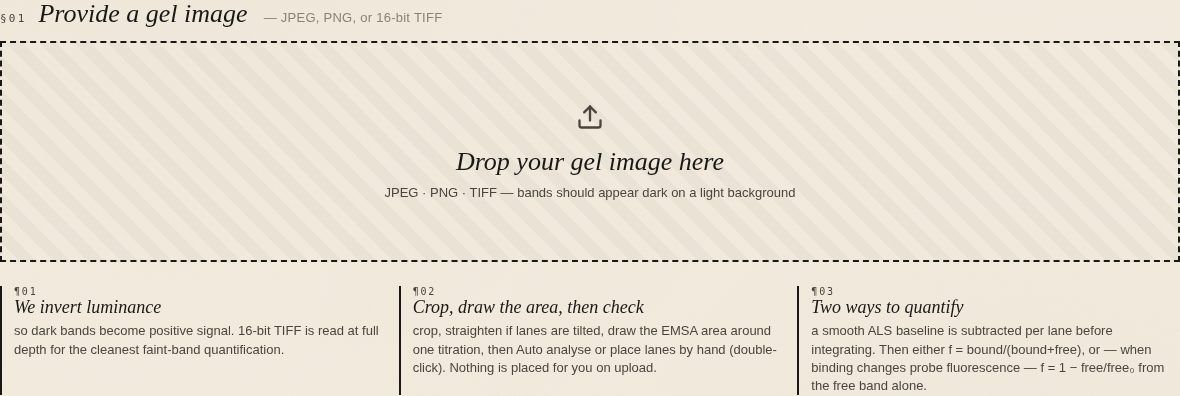
Drop the image on the upload panel, or click it. JPEG, PNG or 16-bit TIFF; dark bands on a light background.

02Crop, and rotate if necessary

Click Crop image and drag a box around the gel so the plate edge is left out. If the lanes are tilted, use the rotate slider — grid lines and a live preview show while you drag, and it is safe at any time, even after lanes are placed. Reset crop brings the full frame back.

Loaded, before cropping — Loaded — whole frame

After cropping to the gel — Cropped to the gel

Shortcut: Auto analyse (under the crop and area buttons) straightens the image a little (at most 2°, relative to any rotation you have set) so each lane runs straight through its own bound and free bands, draws the EMSA area around the lanes and bands (several loadings side by side end up in one area), and detects lanes and bands inside it. If you have drawn an EMSA area yourself it works inside that area instead — do this: without a drawn area the lane and band detection is much less reliable, with it Auto analyse usually gets the whole gel right in one click. Check the result — every step below still applies, and Reset lanes, bands & settings returns to a freshly loaded image (the crop stays).

03Draw the EMSA area around the first titration

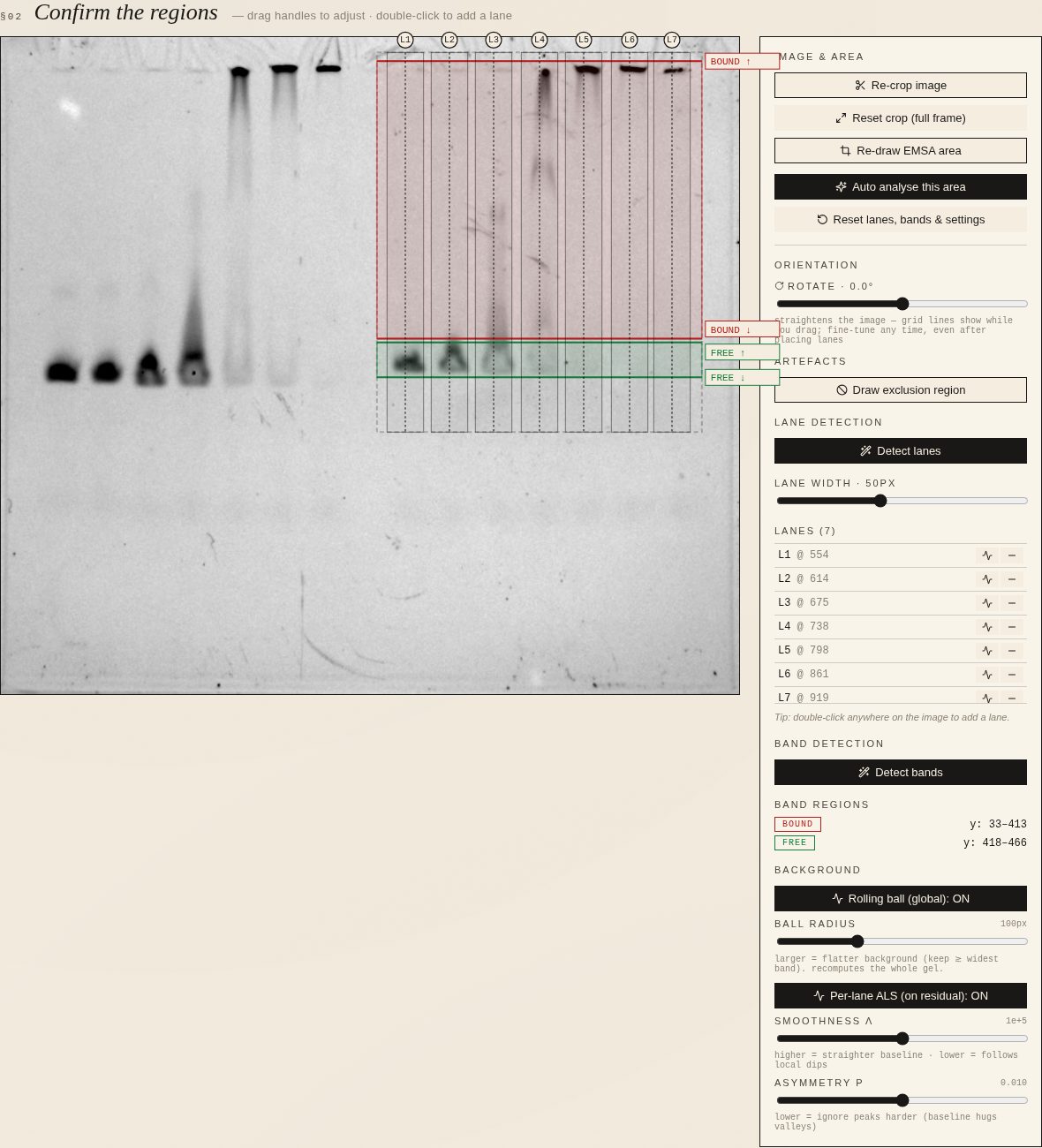
Click Draw EMSA area and drag a box around the lanes of one EMSA, from the wells down past the free probe. Everything you do next — lanes, bands, background — is confined to this area, and the image is not cropped again. The second titration on the same gel is done afterwards by drawing a new area (see below).

EMSA area drawn around the left titration — EMSA area around the left titration

04Exclude artefacts

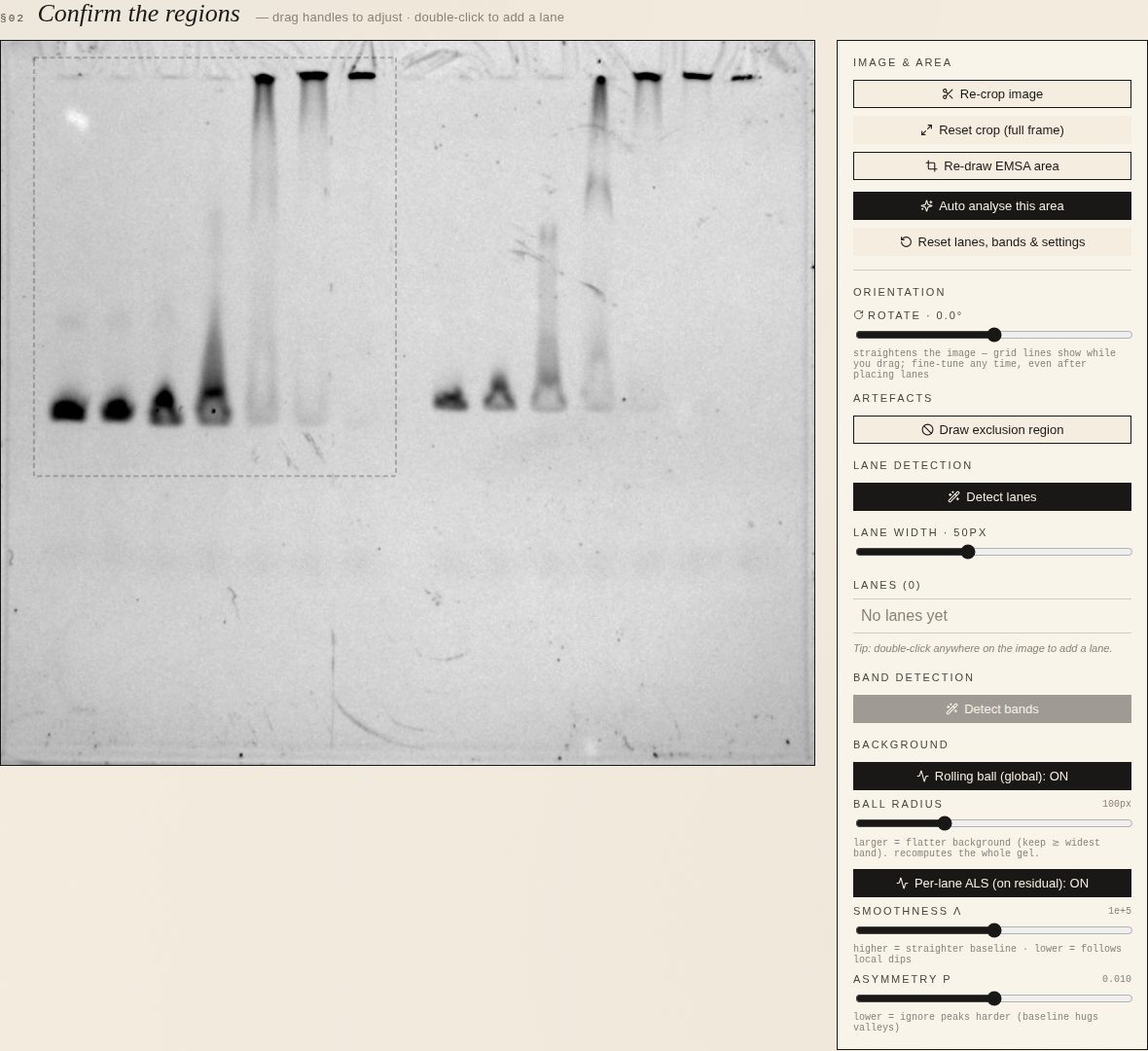
Anything that is not signal — a bubble, a fingerprint, a reflection — should be voided. On this gel there is a pale spot at the top of lanes 1–2. Click Draw exclusion region and drag a box over it; those pixels are dropped from every integration. Draw as many as you need; each is listed under the button with a remove control.

Exclusion region drawn over the reflection at the top of lanes 1 and 2 — Exclusion region (hatched) over the reflection at the top of lanes 1–2

Lanes and bands

05Place lanes

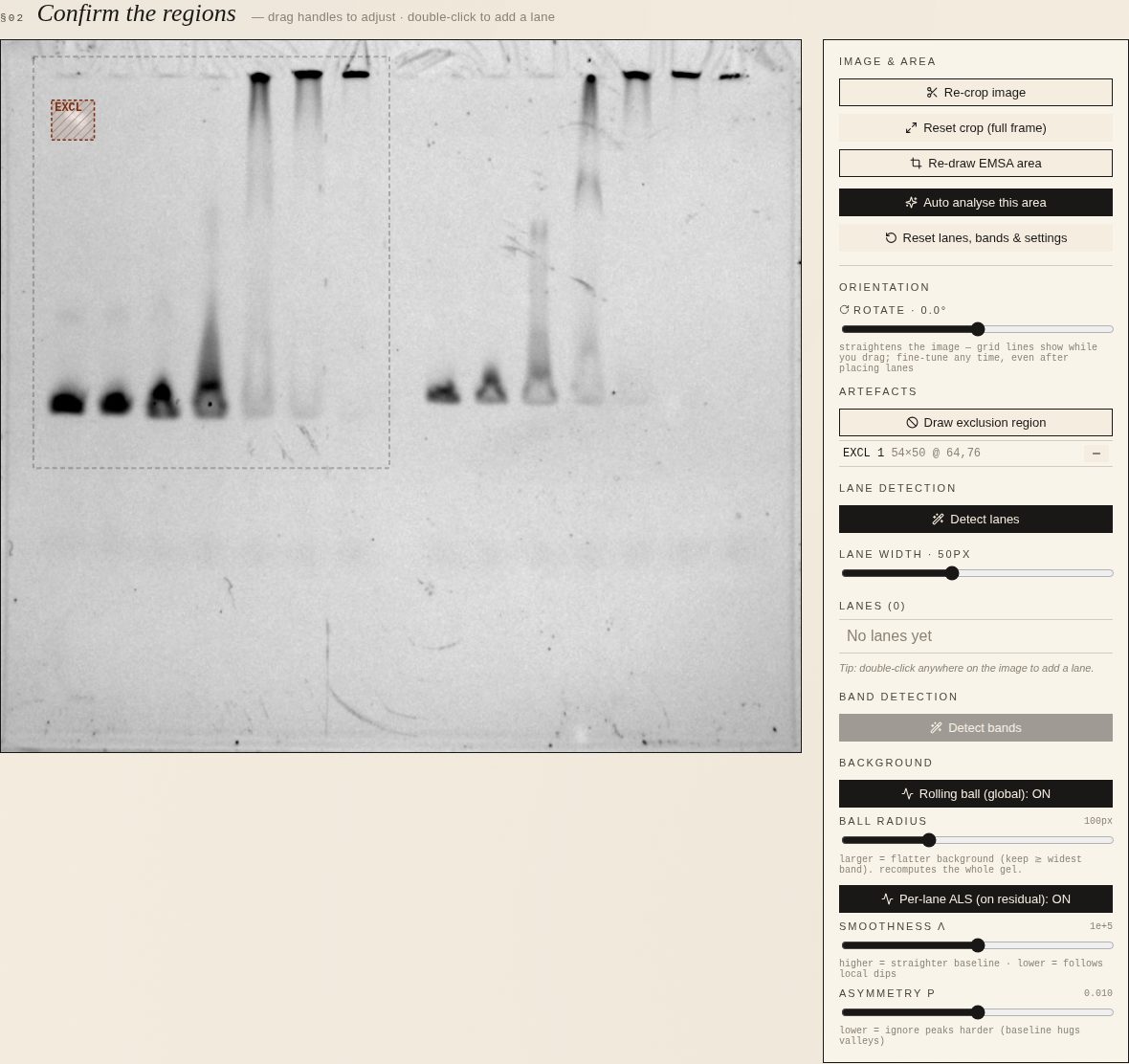
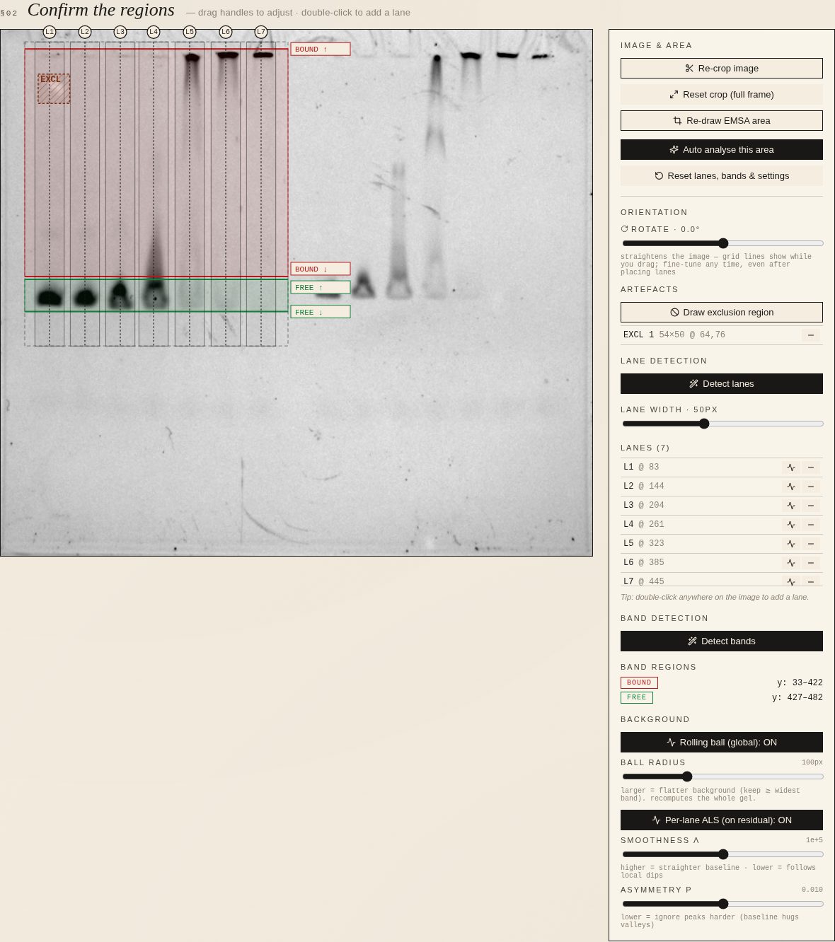
Double-click each lane centre, left to right. Lanes are labelled L1, L2, … and drag by their round handle. Set lane width so the strips cover the bands without overlapping. Remove a lane with its − button.

Detect lanes (or Auto analyse) places evenly spaced lanes inside the EMSA area. It is reliable once the area is drawn; without one, or on gels with smears and bright wells, check the lane count and fix by hand.

06Mark the bound and free windows

Click Detect bands. Two horizontal windows appear: red = bound complex, green = free probe. Drag the BOUND ↑/↓ and FREE ↑/↓ handles so each window encloses its band in every lane. Here the complex sits in the wells and smears beneath them, so the bound window is dragged down to take in the smear, and the free window is tall enough to include the tail above a partially bound band.

Seven lanes placed, bound and free windows adjusted — Seven lanes placed by double-click; bound window covering wells and smear, free window around the probe

Check the background

optional · worth doing once per gel

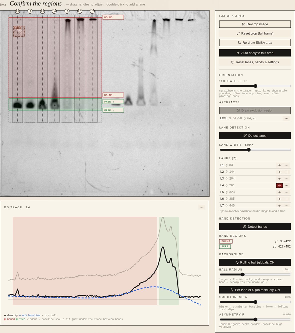
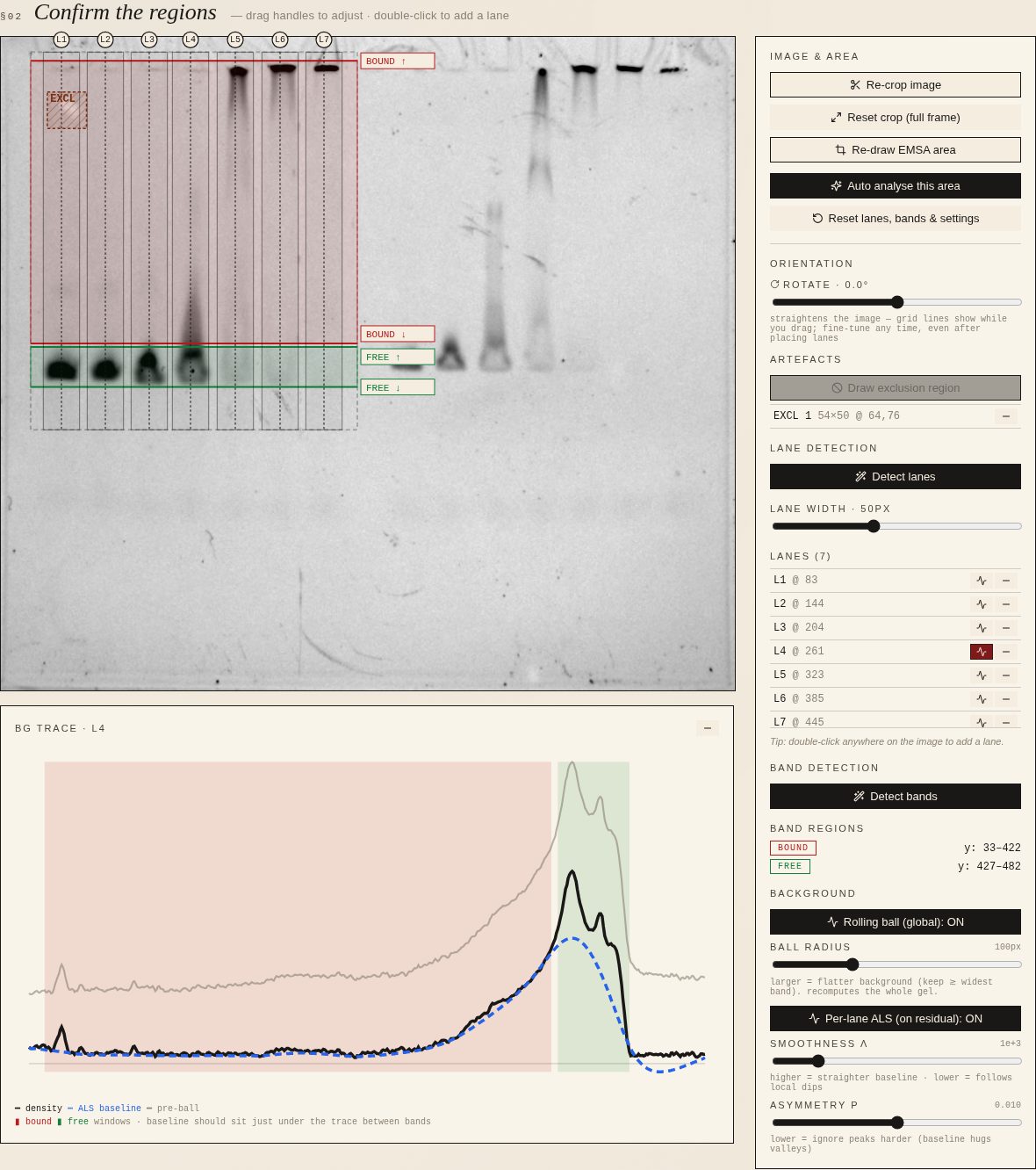
Click the ∿ button next to any lane to open its bg trace: grey = raw density down the lane, black = after the global rolling ball, blue dashed = the per-lane ALS baseline that will be subtracted. The baseline should sit just under the black trace between bands.

Rolling ball (global) removes 2-D illumination gradients over the whole gel. Keep the radius larger than the widest band (default 100 px).
Per-lane ALS fits a smooth baseline under each lane profile. Smoothness λ: higher = straighter (default 1e5). Lowering λ lets the baseline climb into wide bands and eat their signal — the right-hand image shows λ = 1e3 doing exactly that under lane 4's free band. Asymmetry p (default 0.01): lower ignores peaks harder.

When in doubt, leave the defaults.

Background trace for L4 at the default λ = 1e5 — L4 at λ = 1e5 (default) — baseline flat under the band

Same lane at λ = 1e3 — the baseline rises under the band — L4 at λ = 1e3 — baseline rises into the band: wrong

Concentrations and fit

07Enter concentrations

Type the protein concentration for each lane (unit selector on the left; 0 for the no-protein control). [DNA] substrate is only needed for the tight-binding model.

Concentration entry — One field per lane

08Choose how fraction bound is defined, then read the fit

The Quantification & binding fit section appears after three or more concentrations. Two definitions are offered:

Bound / total — bound / (bound + free). Self-normalising per lane, but assumes the label is equally bright in both bands.
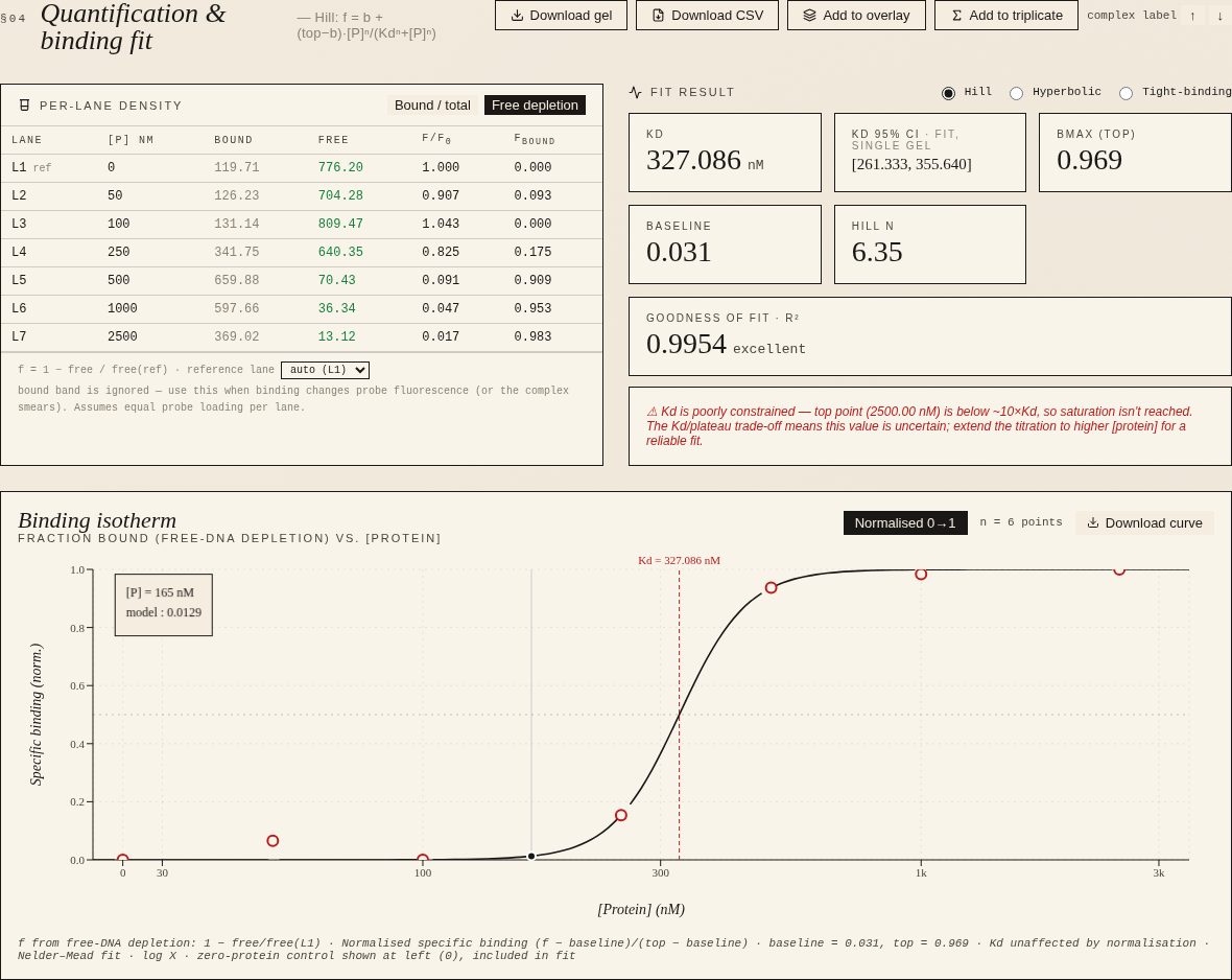
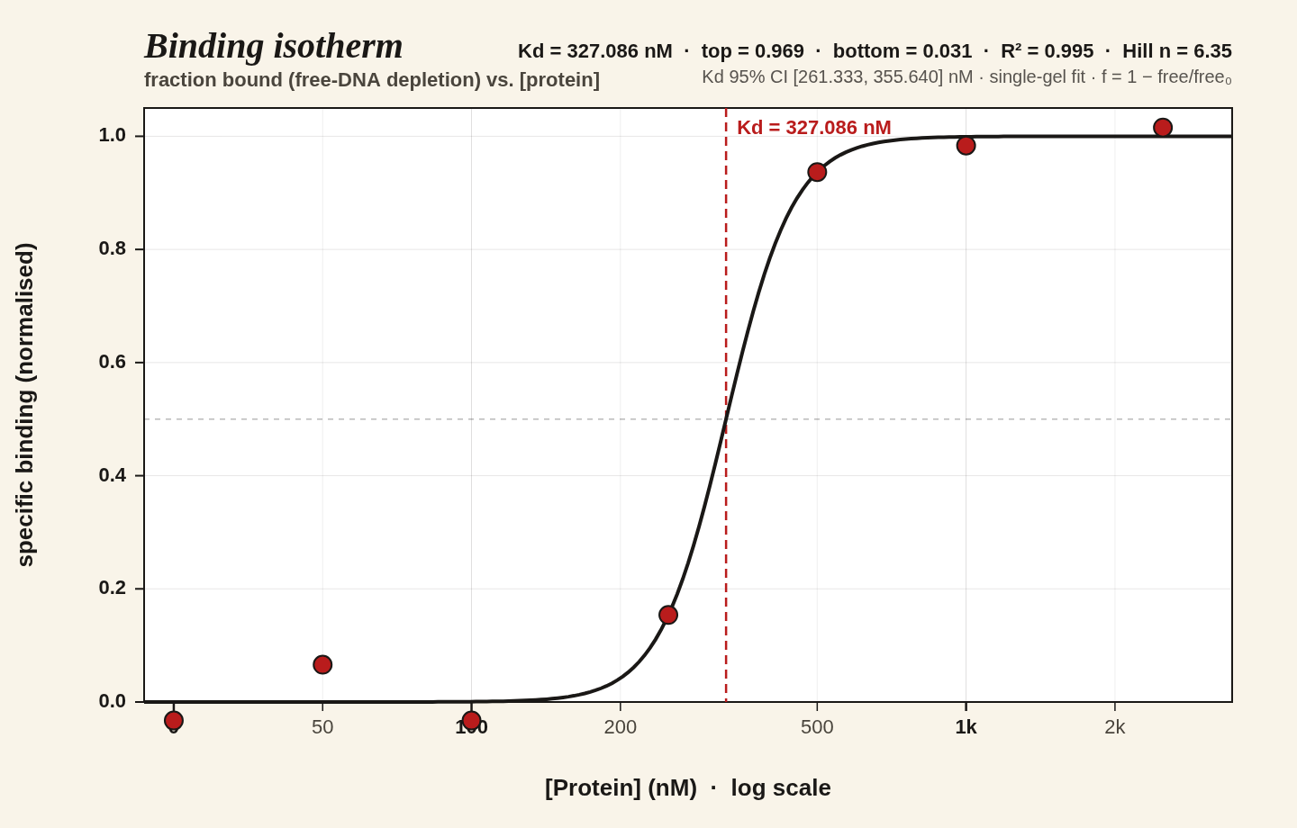
Free depletion — 1 − free / free(reference lane). Reads only the disappearance of the free probe, so it is the right choice when the complex smears, super-shifts or sits in the wells, or when binding changes the probe's brightness.

For this example the complex is in the wells and smears down the lane, so Free depletion is used. The reference lane defaults to the lowest [protein].

Right of the table: K_d, its single-gel bootstrap CI, plateau, baseline, Hill n and R²; below, the isotherm. Hill / Hyperbolic / Tight-binding switches the model.

Read the warnings. “Kd is poorly constrained” means the top concentration is below ~10×K_d, so the plateau is not reached — the number is uncertain however good R² looks.

Fit panel with free depletion selected — Fit panel, free depletion: per-lane table, parameters, isotherm

Export

Download gel — the gel annotated with concentrations and band labels.
Download curve — the isotherm as a PNG with the fit parameters and the fraction definition in the header.
Download CSV — lane, [protein], bound, free, total, fraction_bound.
Add to overlay / Add to triplicate — send this titration to those tabs.

Second EMSA on the same gel

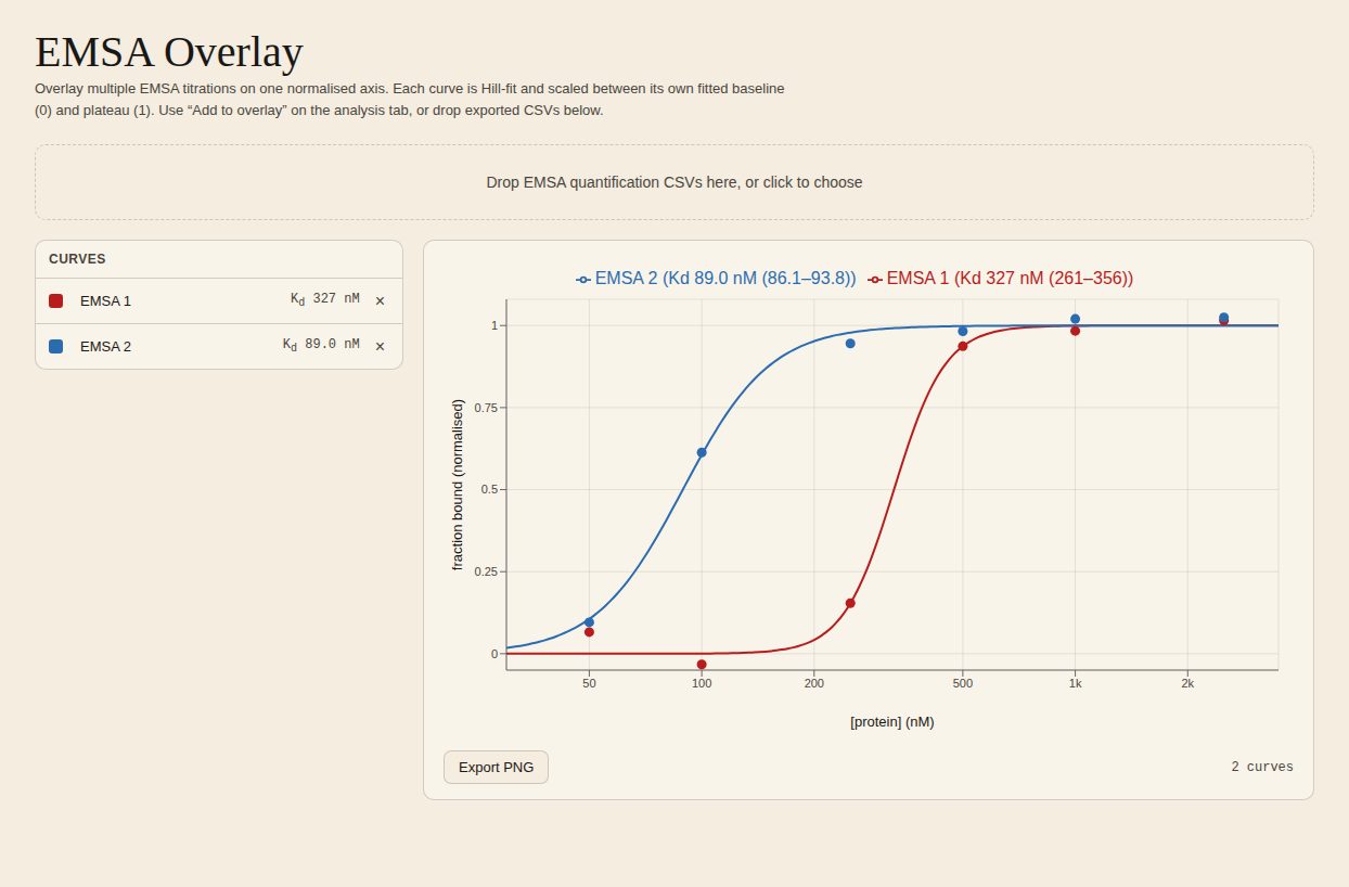
Click Reset lanes, bands & settings (the image and crop stay), then Draw EMSA area around the other titration and repeat from step 04. Send both to Overlay to compare K_d values on one axis.

EMSA area drawn around the right titration with lanes and bands placed — New EMSA area around the right titration

Overlay of the two titrations from the example gel — Overlay tab: both titrations